Understanding LLM Embeddings from Scratch — Part 5: Word2Vec

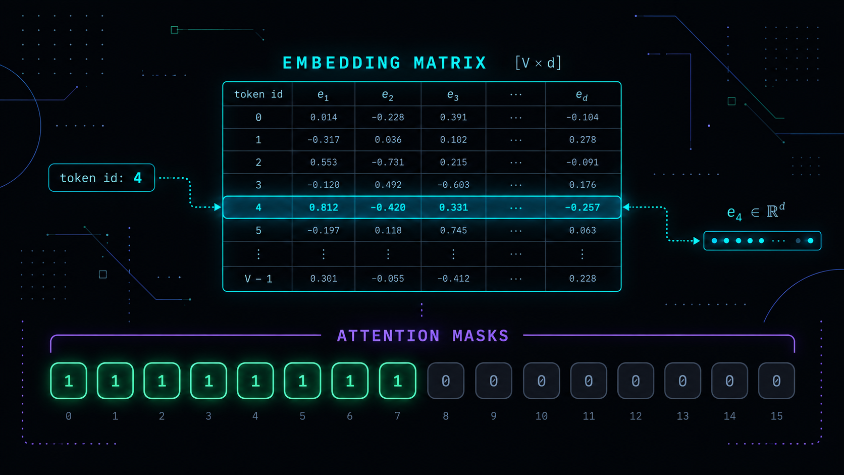
In Module 4, we treated embeddings as raw parameters—numbers in a matrix tuned by backpropagation to minimize a loss value.

Now, we step back from the raw mechanics to look at the emergence of meaning itself.

Today, we explore how simple word co-occurrence gives rise to the famous Word2Vec architecture, how negative sampling turns an impossible probability problem into simple binary classification, and how vector spaces end up capturing real-world relationships.

1. The core idea: You can learn about a word from its neighbors

Imagine you're learning an unfamiliar language. You repeatedly encounter these sentences:

• "The cat eats food."
• "The dog eats food."
• "The cat drinks water."
• "The dog drinks water."
• "The apple grows on trees."
• "The banana grows on plants."

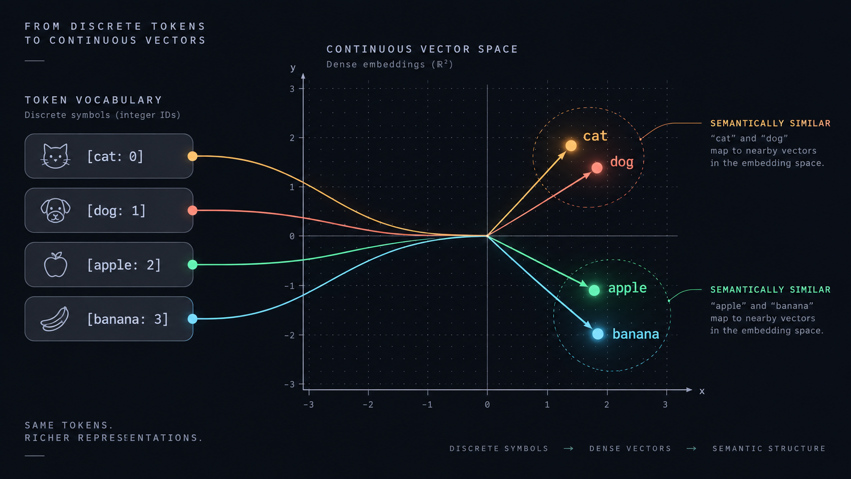
Even without knowing what cat and dog mean, you could observe that they appear in similar linguistic contexts. Meanwhile, apple and banana frequently appear in a different set of contexts.

Words occurring in similar contexts often have similar meanings or linguistic roles.

How can we represent this mathematically?

Suppose we count how frequently different words appear near each target word.

For example a sample table,

Word	eats	drinks	grows	ripe
cat	8	7	0	0
dog	7	8	0	0
apple	0	0	8	7
banana	0	0	7	8

Invented counts for teaching. Each row records how often the word appeared with each context feature.

For cat, this table gives us:

$$\mathbf v_{\text{cat}}=[8,7,0,0]$$

For dog:

$$\mathbf v_{\text{dog}}=[7,8,0,0]$$

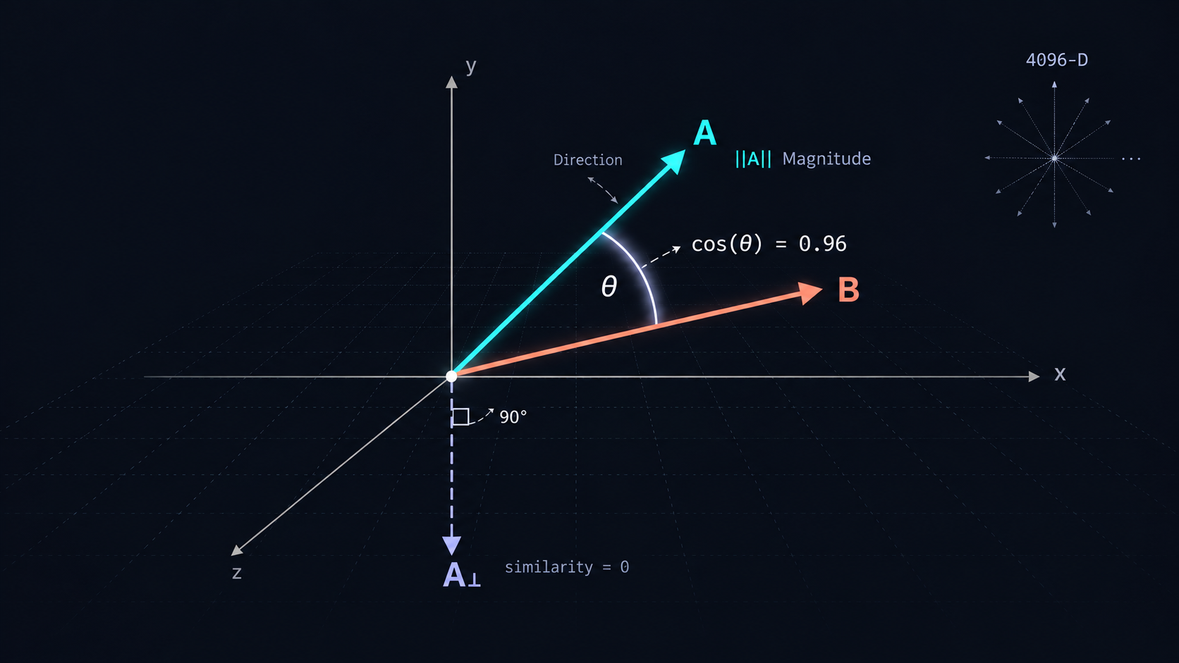
These vectors are similar because the words have similar context patterns.

But apple has:

$$\mathbf v_{\text{apple}}=[0,0,8,7]$$

This is different. The interesting thing is that we didn't encode the concept of "animal" anywhere. We only counted what appeared around each word. Yet the resulting numerical patterns can reveal meaningful groupings.

2. Let's measure the similarity

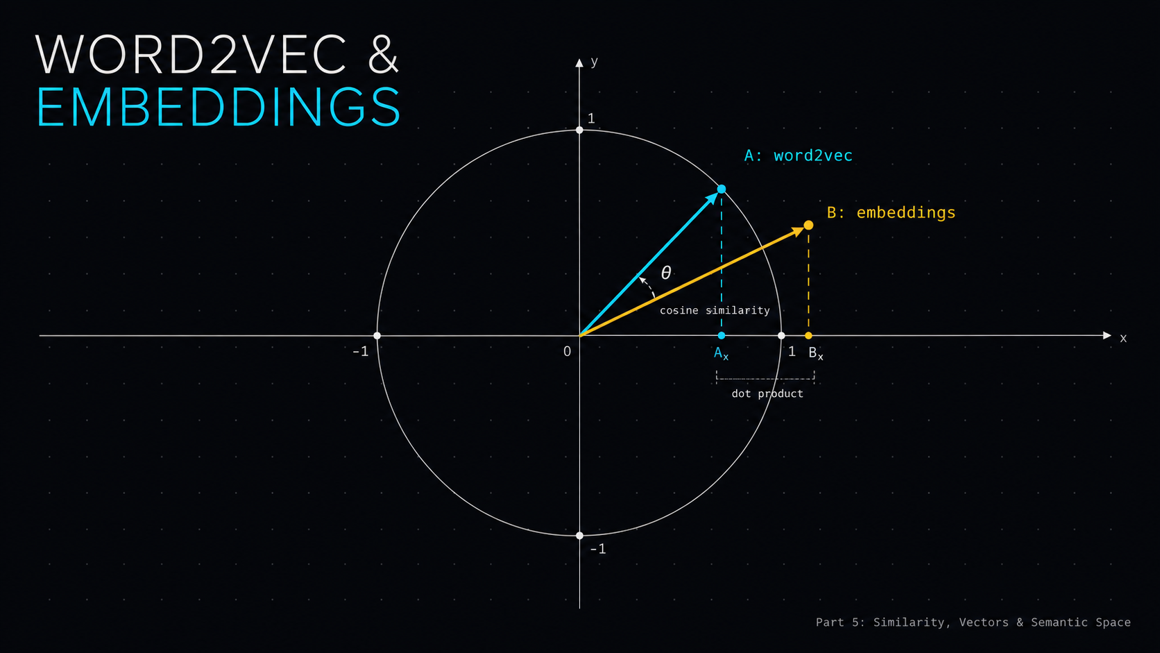
We already learned cosine similarity in Module 2.

$$\operatorname{cosine}(A,B)= \frac{A\cdot B}{|A||B|}$$

For cat and dog:

Their dot product and cosine similariry is:

import torch
import torch.nn.functional as F

cat = torch.tensor([8.0,7.0,0.0,0.0])
dog = torch.tensor([7.0,8.0,0.0,0.0])

dot_product = torch.dot(cat, dog)

print(dot_product)

cosine = F.cosine_similarity(
    cat.unsqueeze(0),
    dog.unsqueeze(0),
    dim=1
)

print(cosine)

# tensor(112.)
# tensor([0.9912])

Now compare cat and apple.

apple = torch.tensor([0.0, 0.0, 4.0, 7.0])

# dot and cosine between cat and apple
dot_product_cat_apple = torch.dot(cat, apple)

cosine_cat_apple = F.cosine_similarity(
    cat.unsqueeze(0),
    apple.unsqueeze(0),
    dim=1
)

print(dot_product_cat_apple)
print(cosine_cat_apple)

# tensor(0.)
# tensor([0.])

This gives us our first important insight:

Meaning-like structure can emerge from statistical patterns in language, without manually assigning meanings to the dimensions.

However, our approach has a limitation. If we had a vocabulary with 100,000 possible context words, our context-count vector could require 100,000 dimensions. It would also be extremely sparse.

Can we learn a much smaller vector that preserves useful information from these patterns? That's where Word2Vec comes in.

3. Word2Vec: Learn dense vectors by predicting context

Word2Vec is a family of neural word-embedding methods introduced in 2013. Instead of manually building a giant word-context count table, we train a small predictive model. The model learns dense embeddings as a byproduct of its prediction task.

There are two important Word2Vec approaches.

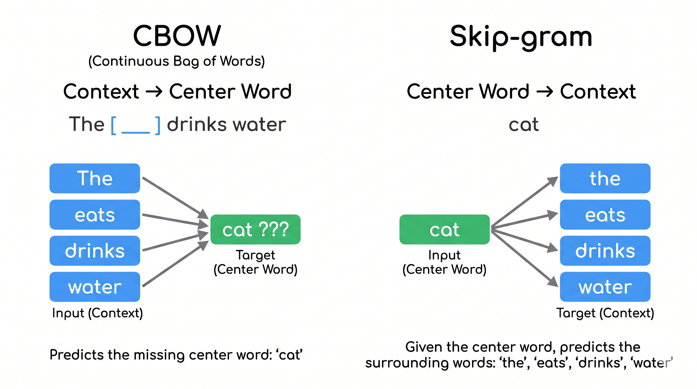
• CBOW (Continuous Bag of Words): Looks at the context words and guesses the blank: Eg: The [ ___ ] drinks water --> predicts cat.
• Skip-gram: Takes the center word and predicts its surroundings: cat --> predicts [the, eats, drinks, water].

Let's take the sentence:

"the small cat drinks water"

Assume a context window of two positions.

The center word is cat.

Its context words are:

the, small, drinks, water

Skip-gram creates four training pairs:

("cat", "the")
("cat", "small")
("cat", "drinks")
("cat", "water")

CBOW instead takes the surrounding words as inputs and predicts cat.

Why does this create embeddings?

Think about Skip-gram. To predict the context words around cat, the model must develop a useful internal representation of cat. To predict context words around dog, it faces many similar requirements.

Because the prediction system shares parameters across words, the model can benefit from developing related representations for words with similar contexts.

This is not an explicit similarity rule. It is a consequence of optimizing the prediction task.

4. Negative sampling: How does the model know which contexts are wrong?

Let's think about what Skip-gram is trying to do.

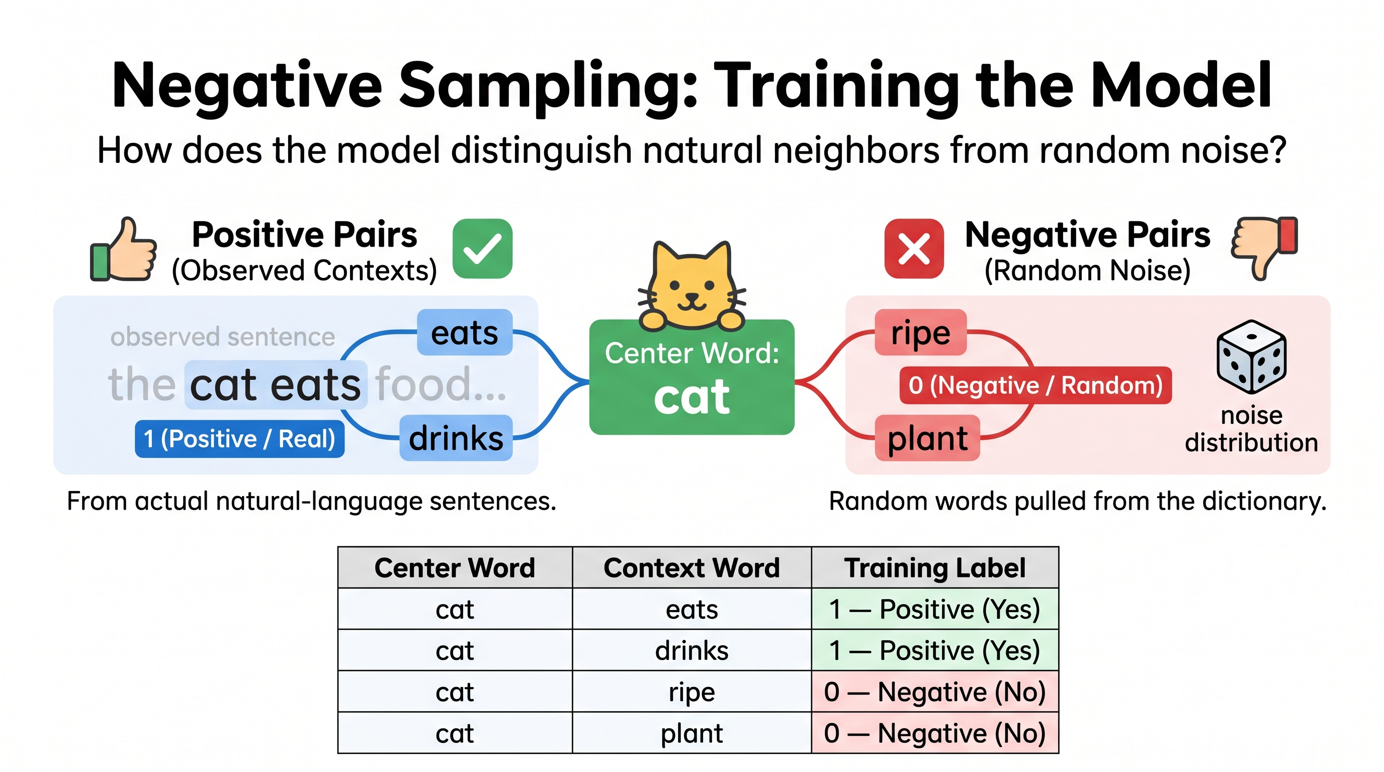
For the center word cat, we want the model to recognize that eats is a likely context word.

But we also need it to distinguish eats from randomly selected, less appropriate context words such as ripe.

We can construct two kinds of examples:

Center word	Context word	Training label
cat	eats	1 — Positive
cat	drinks	1 — Positive
cat	ripe	0 — Negative
cat	plant	0 — Negative

Positive pairs come from observed word-context co-occurrences.

Negative pairs are sampled from a noise distribution, rather than requiring someone to manually label every pair.

Why not just use softmax over the entire vocabulary?

Suppose our vocabulary contains 100,000 words. To predict a context word with a full softmax, we'd calculate a score for every one of those 100,000 vocabulary entries. That's expensive.

Instead, negative sampling asks a simpler question:

Does this center word and context word pair look like a real co-occurrence or a randomly sampled pair?

For each positive pair, we might sample five negative pairs. That means we calculate scores for six pairs rather than all 100,000 possible context words. This is one reason negative sampling made Word2Vec practical for large datasets.

5. The mathematics of negative sampling

Let's build this from the embedding vectors.

Suppose we have:

$$u_{\text{cat}}=[0.4,0.2]$$

This is our input embedding for cat.

And two output/context embeddings:

$$v_{\text{eats}}=[0.6,0.1]$$

$$v_{\text{ripe}}=[-0.3,0.2]$$

Notice that Word2Vec Skip-gram with negative sampling has two embedding matrices:

• An input embedding matrix for center words.
• An output embedding matrix for context words.

This is different from our simplified Module 4 model, where we focused on one embedding matrix and a linear prediction layer. Mathematically, however, the ideas are closely related.

Step 1: Calculate a compatibility score

We use the dot product:

$$s=u_{\text{center}}\cdot v_{\text{context}}$$

For the positive pair (cat, eats):

$$s_+=(0.4)(0.6)+(0.2)(0.1)=0.26$$

For the negative pair (cat, ripe):

$$s_-=(0.4)(-0.3)+(0.2)(0.2)=-0.08$$

Step 2: Convert scores into probabilities

Instead of softmax, negative sampling uses the sigmoid function:

$$\boxed{\sigma(x)=\frac{1}{1+e^{-x}}}$$

It converts any real-valued score into a number between 0 and 1.

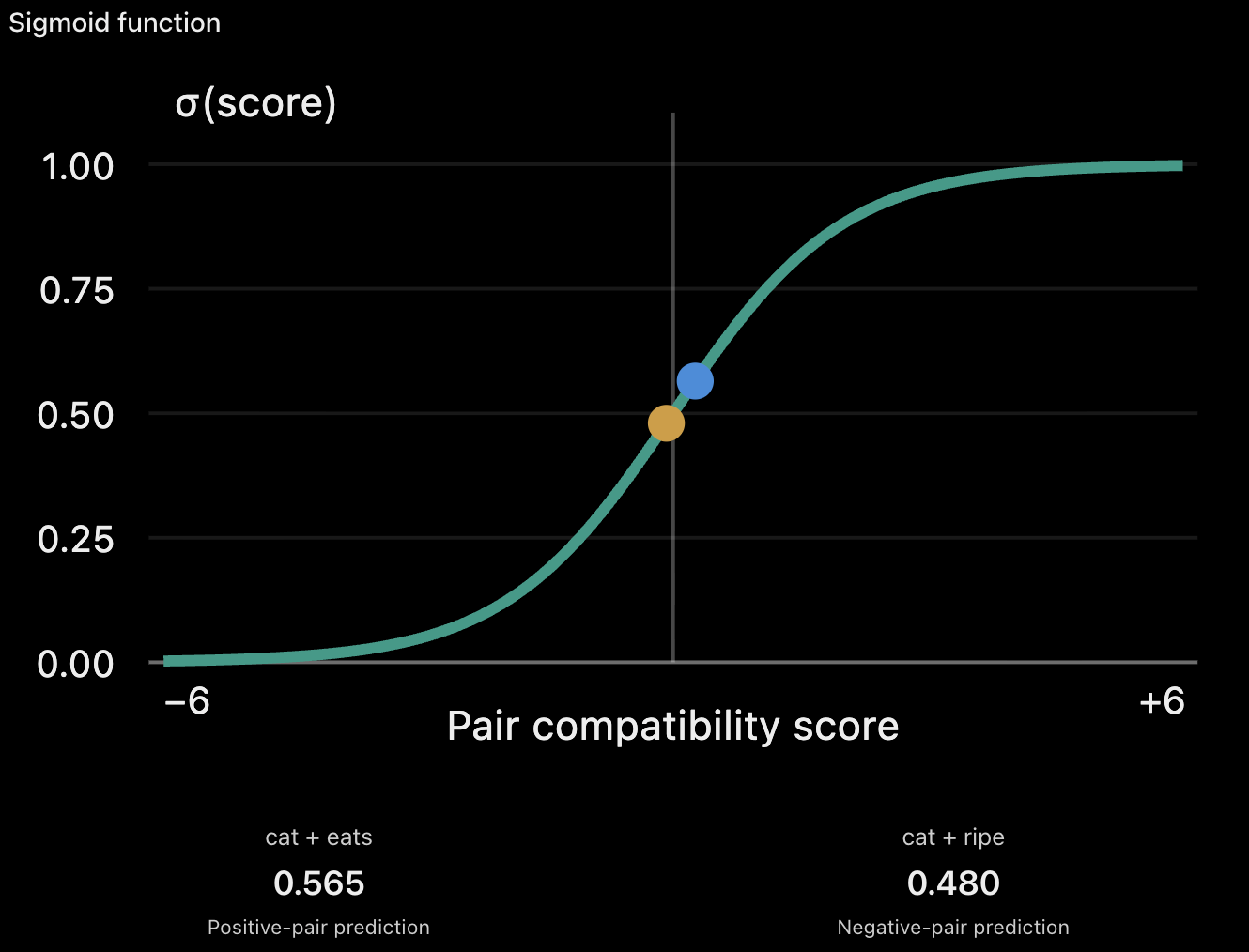
Our positive pair gets a score above 0.5, but not by much and our negative pair gets a score below 0.5, but again, not by much.

We want training to push them further apart.

Step 3: Define the negative-sampling loss

For one positive pair and one negative pair:

$$\boxed{ L=-\log \sigma(s_+)-\log \sigma(-s_-) }$$

Let's understand the two terms.

Positive term:

$$-\log\sigma(s_+)$$

We want \(s_+\) to become large and positive so \(\sigma(s_+)\) approaches 1.

Negative term:

$$-\log\sigma(-s_-)$$

We want \(s_-\) to become very negative so \(\sigma(-s_-)\) approaches 1.

In our example:

$$L=-\log(0.565)-\log(0.520)$$

$$\boxed{L\approx1.2255}$$

The general loss with $k$ negative samples is:

$$\boxed{ L=-\log\sigma(u\cdot v_+) -\sum_{j=1}^{k}\log\sigma(-u\cdot v_j^-) }$$

This is the central training objective of Skip-gram with Negative Sampling.

Step 4: How do gradients update the embeddings?

Here's the connection to Module 4.

For our one-positive, one-negative example, the gradient with respect to the center embedding $u$ is:

$$\frac{\partial L}{\partial u} = (\sigma(s_+)-1)v_+ + \sigma(s_-)v_-$$

Substitute the numbers:

$$=(0.5646-1)[0.6,0.1]+0.4800[-0.3,0.2]$$

$$\boxed{ \frac{\partial L}{\partial u} \approx[-0.4052,0.0525] }$$

With learning rate 0.1:

$$u_{\text{new}}=u_{\text{old}}-0.1\nabla_u L$$

$$=[0.4,0.2]-0.1[-0.4052,0.0525]$$

$$\boxed{u_{\text{new}}\approx[0.4405,0.1948]}$$

The context embeddings also receive gradients and are updated.

Over many examples, these updates encourage observed word-context pairs to have higher dot products and sampled negative pairs to have lower dot products.

This is how the training objective gradually organizes the embedding space.

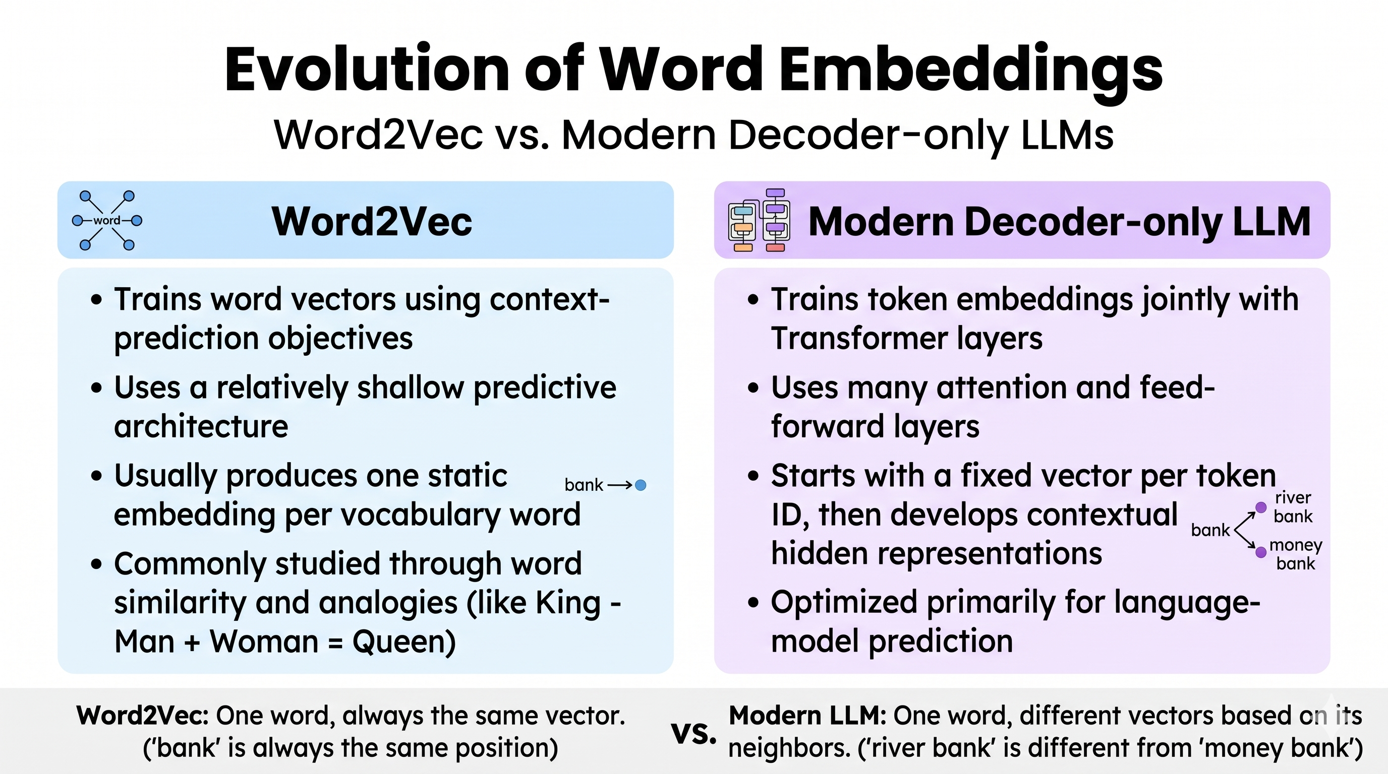
Consider these two sentences again:

• "I went to the bank to withdraw money."
• "I sat beside the river bank." A static Word2Vec embedding typically gives bank one vector regardless of its usage.

A Transformer starts with a token embedding and then processes the surrounding context, producing different hidden representations. That allows the system to distinguish different meanings and usages of the same token. This is one of the biggest conceptual differences between traditional word embeddings and contextual representations.