


Introduction
Bias and Variance are the two most important concepts in the field of Machine Learning. These help us to understand the performance of the model. You’ve probably heard of terms like Bias-variance trade-off, bias-variance decomposition, etc. In this article, we are decoding these terms in a simplified way.
But before that, let’s talk about errors in Machine Learning.
In machine learning, errors can be classified into two categories: reducible errors and irreducible errors.
Reducible Errors: These errors can be minimized or reduced by improving the model complexity. Reducible errors are typically caused by factors such as bias or variance in the model which we will understand soon.
Irreducible Errors: These types of errors are present in the data because of the noise and randomness. These errors cannot be modelled.
As we cannot decrease the irreducible errors, we have to play with Reducible errors. And here, the concept of Bias and Variance comes in.
What is Bias?
Simply put, Bias is the error between the average prediction value given by a ML model and the actual/expected value. A model with high bias tends to underfit the data. It means the model is too simple to understand the underlying pattern of the data. Because of this, the model performs poorly on training and testing data.
Machine Learning Algorithms with Low Bias: Decision Tree, K-Nearest Neighbours, etc.
Machine Learning Algorithms with High Bias: Linear Regression
What is Variance?
Variance, on the other hand, refers to the error that is introduced by the model's sensitivity to small fluctuations in the training data. A model with high variance is typically too complex and may overfit the training data, meaning it performs well on the training set but poorly on the test set.
Machine Learning Algorithms with Low Variance: Linear Regression
Machine Learning algorithms with High Variance: Decision Tree, K-Nearest Neighbours, etc.
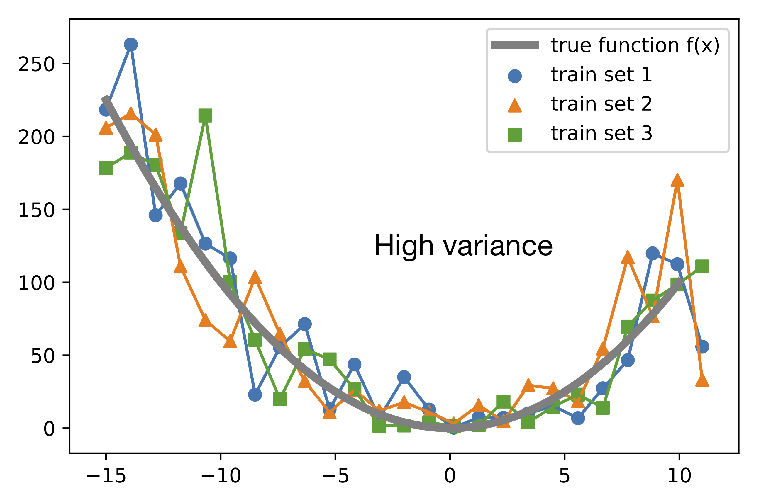
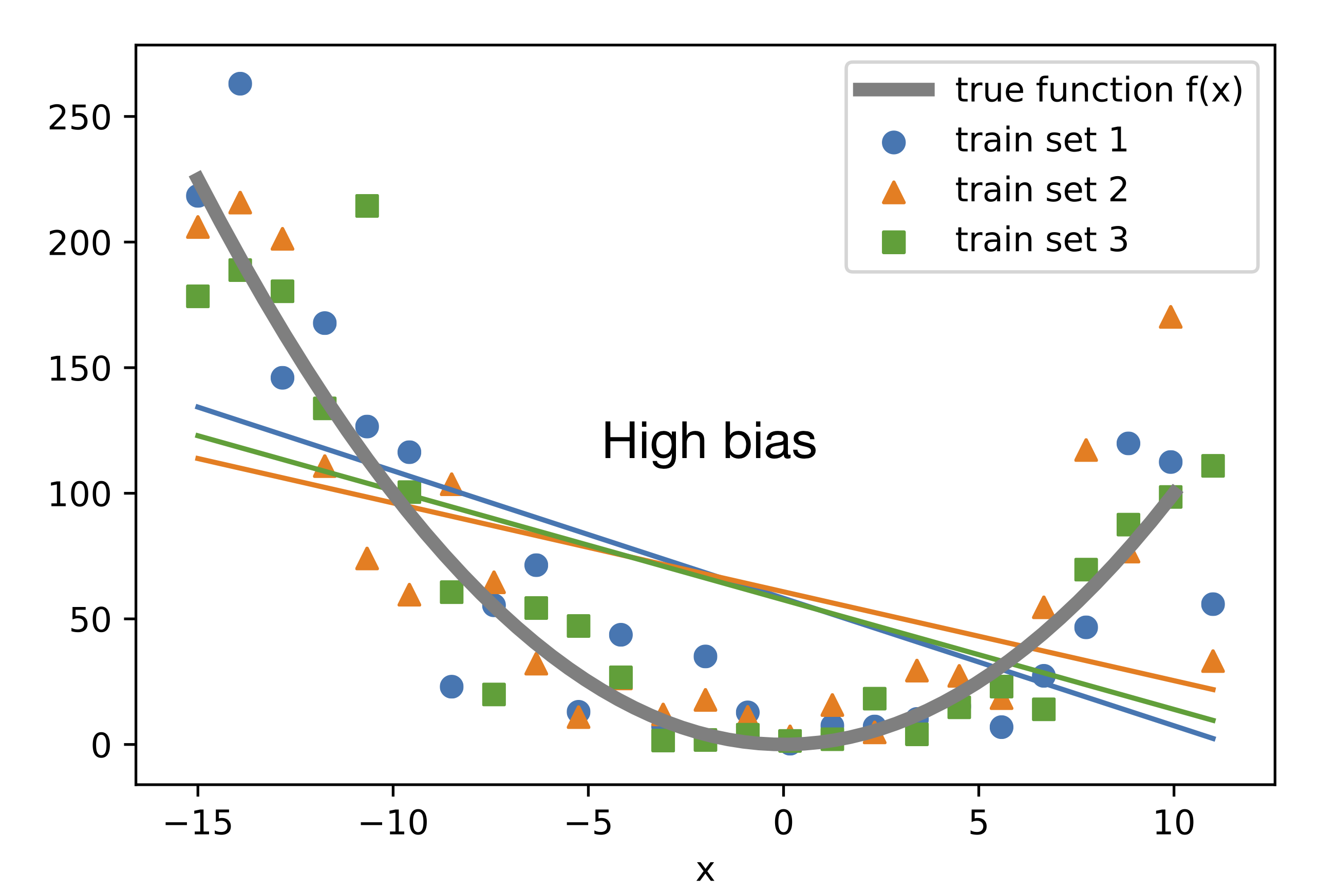
Notice these three images.

In the first one, the red line tries to touch all the points in the dataset. It means it pays a lot of attention to the training data which leads to overfitting. As a result, a model with high variance works well on the training data but failed to perform on the testing/unseen data.
In the second image, you can clearly see, the data is non-linear but the model draws simply a linear line. This is due to high bias and results underfitting. The model oversimplifies the dataset. It always leads to high errors in both training and testing dataset.
Now look at the third image. In machine learning, we try to find a balance between bias and variance. A model with high bias and low variance may be too simple, while a model with low bias and high variance may be too complex. The ideal model has low bias and low variance, meaning it is able to capture the underlying patterns in the data without overfitting.
Different Combinations of Bias and Variance:
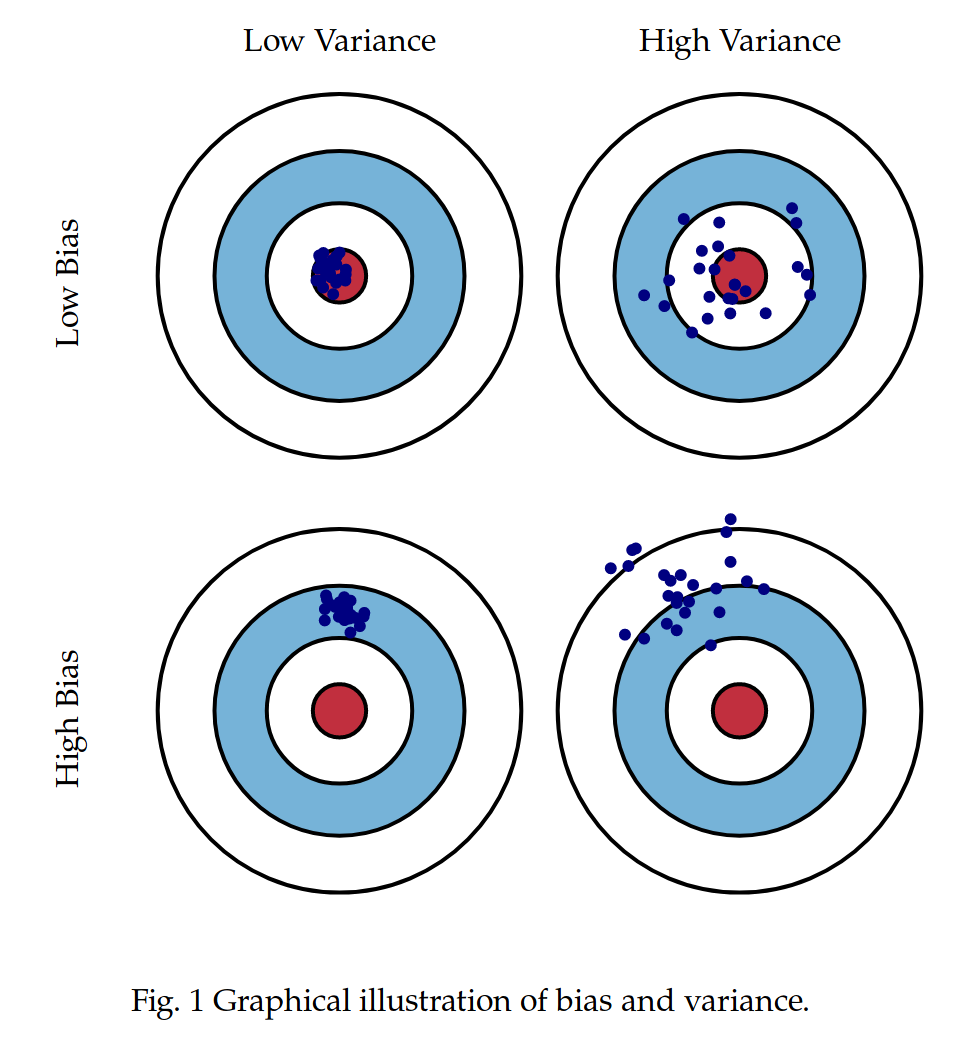
Low Bias – Low Variance: This is the ideal situation. It means the model is able to capture the true function of the data without overfitting.
Low Bias – High Variance: In this scenario, the model learns a lot of things from a particular training dataset. It fails to perform on the test dataset and leads to overfitting.
High Bias – Low Variance: In this case, the ML algorithm oversimplifies the model, and gives poor prediction.
High Bias – High Variance: This is the worst scenario. Here, the model gives inaccurate predictions in different datasets.
Bias–Variance Trade-off:
If our model is too simple and has very few parameters then it may have high bias and low variance. On the other hand, if our model is complex and has a large number of parameters then it’s going to have high variance and low bias. So, we need to find the right/good balance without overfitting and underfitting the data.
For the ideal model, we have to make sure that bias and variance both should be low. But, in reality,
When we decrease bias, the variance will increase
When we decrease the variance, the bias will increase
And because of this Bias-Variance Trade-off, we need a generalized model. So, we need to find a sweet spot between bias and variance to make an optimal model.

Bias-Variance Decomposition:
Bias-variance decomposition is a concept used to analyse and understand the expected error of a machine learning model. It breaks down the overall error into three components:
Total Error = Bias² + Variance + Irreducible Error
Imagine you have an ML algorithm that trains a model to make predictions based on a given dataset. The true relationship between the input features and the target variable is often unknown, and the goal is to learn an approximation of this relationship using the available data (sample data).
The bias-variance decomposition provides insights into how the model's predictions differ from the true values. Let's break it down step by step:
True Relationship: This represents the actual, underlying relationship between the input features and the target variable in the data. In most cases, we don't know this true relationship, but we aim to approximate it with our model.
Expected Prediction: The expected prediction is the average prediction that our model would make over many different training sets. Since the training data is often a sample from the true distribution, we can think of this as the prediction we would make if we had access to an infinite amount of data.
Bias: Bias is the error between the expected prediction and the true relationship. It captures how much the model's predictions differ, on average, from the true values, regardless of the training set. A high bias indicates that the model is too simplistic or unable to capture the complexity of the data. It tends to underfit the data and overlook important patterns or relationships.
Variance: Variance represents the variability of the model's predictions across different training sets. It measures how much the predictions would change if we were to train the model on different subsets of the data. A high variance indicates that the model is overly sensitive to the specific training data and is likely to overfit. It may memorize the training examples instead of capturing the general underlying patterns.
Total Error: The total error of the model can be decomposed as the sum of the squared bias, variance, and an irreducible error component. The irreducible error represents the noise or randomness inherent in the data that cannot be reduced by any model.
Conclusion:
The bias-variance trade-off arises from the fact that reducing bias often leads to an increase in variance, and vice versa. A complex model with low bias can capture true relationships in the data but may have high variance, resulting in overfitting. Conversely, a simple model with high bias may have low variance, but it may not be expressive enough to capture the true underlying patterns.
The goal of machine learning is to strike a balance between bias and variance. We aim to find a model that is complex enough to capture the important patterns in the data (low bias) but not overly sensitive to minor fluctuations or noise in the training data (low variance). This balance is crucial to achieving good generalization performance on unseen data.
By understanding the bias-variance decomposition, we can diagnose and address issues in our models. If the model has a high bias, we can consider increasing its complexity, and adding more features. If the model has high variance, we can employ regularization techniques, or gather more data.