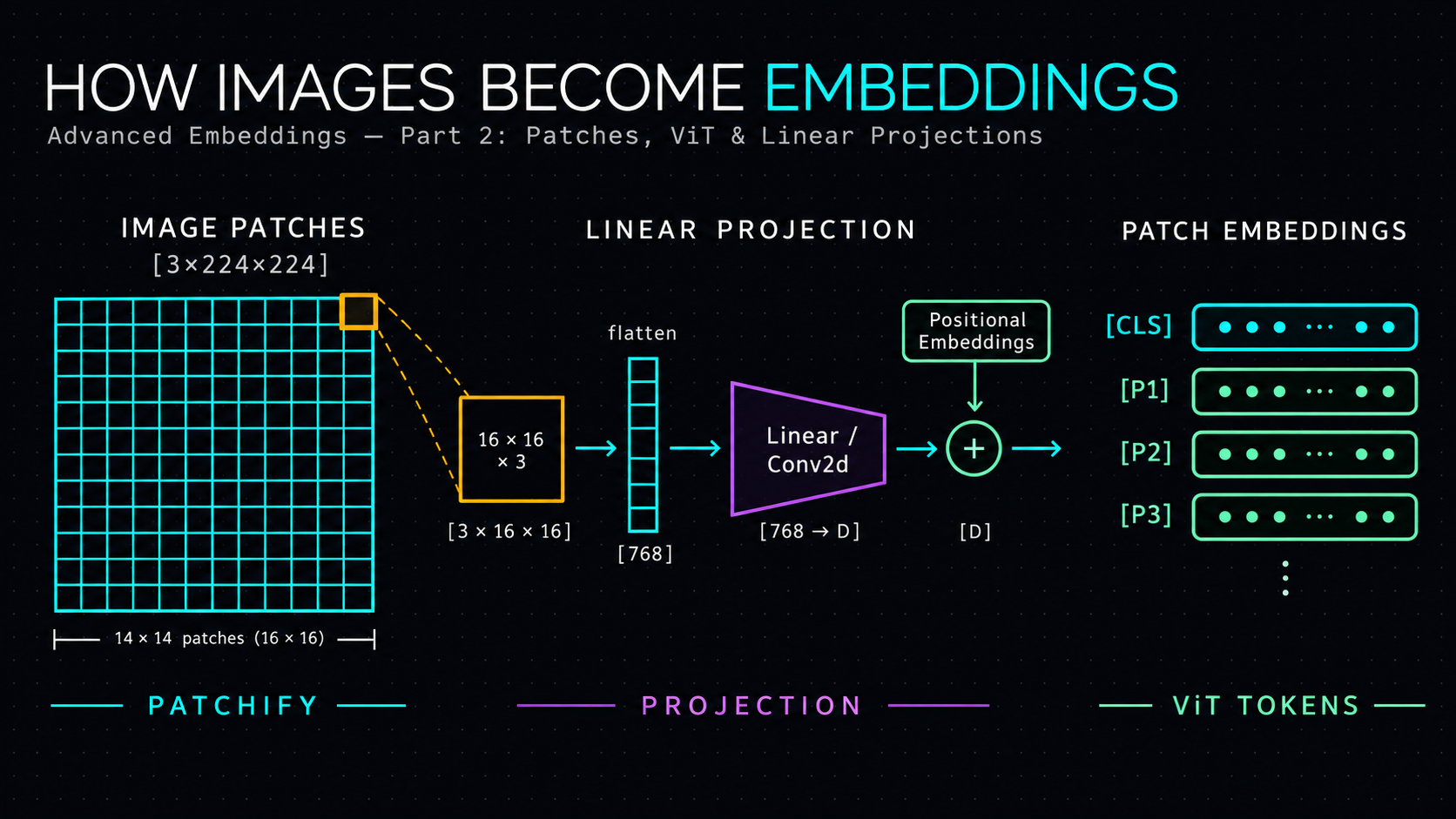
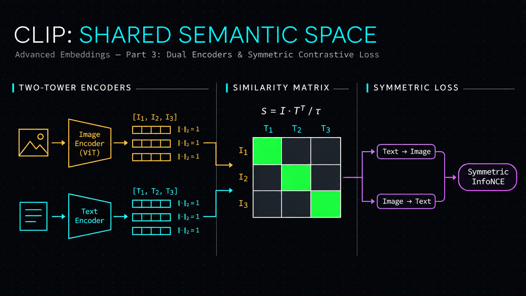
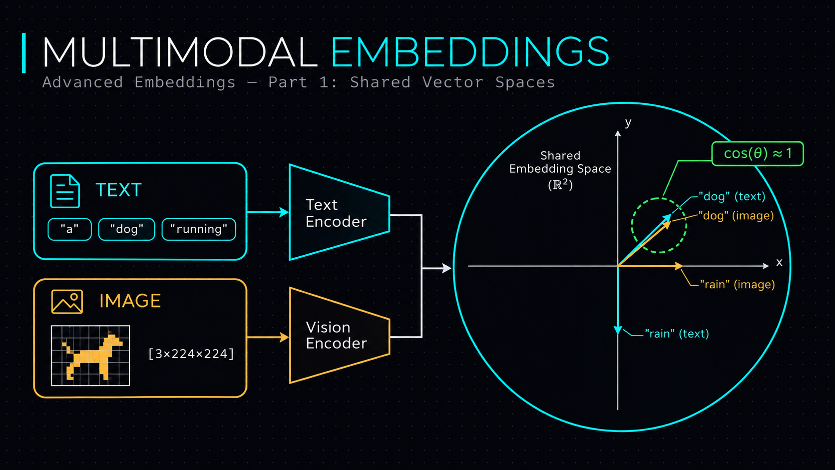
In Module 1, we learned that multimodal models can represent text and images in a shared embedding space. We also learned how contrastive learning encourages matching text-image pairs to have compatible representations. But we left one important component unexplained:

How does an image encoder convert millions of pixel values into a meaningful vector?

We already understand how text embeddings work:

$$\text{Text}\rightarrow\text{Token IDs}\rightarrow\text{Token Embeddings}$$

But images don't naturally contain token IDs. So how do we create something equivalent to tokens for images?

First, what does a computer actually see in an image?

Consider this photograph.

You and I see a dog running on grass. But a computer initially sees something very different: numbers representing pixel intensities.

A digital color image typically has three channels:

• R: Red
• G: Green
• B: Blue

Each pixel contains three values.

For a conventional 8-bit RGB image, those values range from 0 to 255.

For example:

[255,0,0] represents pure red.

[0,255,0] represents pure green.

[0,0,255] represents pure blue.

One pixel is represented by three channel values. A complete image contains many such pixels arranged spatially.

What about an entire image?

Suppose the image dimensions are:

$$224\times224$$

That's:

$$224\times224=50{,}176\text{ pixels}$$

With three color channels:

$$3\times224\times224=150{,}528$$

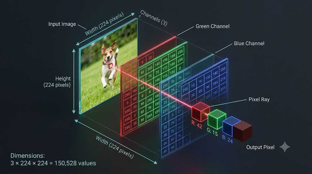
So the raw RGB tensor contains 150,528 numbers.

In PyTorch, we commonly represent an image as:

$$\boxed{X\in\mathbb{R}^{3\times224\times224}}$$

The dimensions are:

[Channels, Height, Width]
   3       224    224

PyTorch: Create an image tensor

import torch

# Simulate one 224x224 RGB image
image = torch.randint(
    low=0,
    high=256,
    size=(3, 224, 224),
    dtype=torch.uint8
)

print(image.shape)
# torch.Size([3, 224, 224])

print(image.numel())
# 150528

Most neural image pipelines then convert the image into floating-point numbers and normalize it.

For example:

image = image.float() / 255.0

print(image.min(), image.max())

The values now lie between 0 and 1.

Real pretrained models may require additional channel-wise normalization using specific means and standard deviations.

Important: These pixel values are not yet semantic embeddings. They're simply numerical measurements of the image.

Why do we need image patches?

You may ask that can we treat every pixel as a token?

In principle, we could. For a 224×224 image, we would have 50,176 pixel positions.

Remember Module 6 from our original series. In standard self-attention, the Query-Key score matrix has shape:

$$QK^\top\in\mathbb{R}^{S\times S}$$

Here, $S$ is the sequence length.

If every pixel becomes a token:

$$S=50{,}176$$

The attention matrix would contain:

$$50{,}176^2 =\boxed{2{,}517{,}630{,}976}$$

That's approximately 2.52 billion scores for a single attention head!

At four bytes per FP32 score, explicitly storing that matrix would require approximately 10.1 GB. And that's just one attention-score matrix, not the entire model. Optimized attention algorithms can avoid materializing that full matrix, but the standard dense attention computation still has quadratic pairwise work.

We need a more manageable representation.

The idea: Divide the image into patches

Instead of treating every pixel independently, we divide the image into small, fixed-size regions called patches. This is a foundational idea in the Vision Transformer (ViT) architecture.

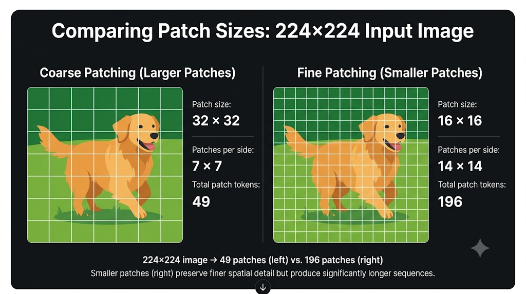
For example, consider a 224×224 image with patches of size:

$$16\times16$$

Along each dimension:

$$224/16=14$$

So there are 14 patches horizontally and 14 vertically.

Total:

$$\boxed{N=14\times14=196\text{ patches}}$$

Instead of processing 50,176 pixel positions as separate tokens, we can process 196 patch tokens.

Why not make patches extremely large?

Suppose we used one patch for the entire image. We'd have just one image token, but we'd lose the opportunity for standard attention to directly model relationships between separate spatial regions. On the other hand, tiny patches produce longer sequences and greater computational cost.

So patch size creates a tradeoff between spatial detail and efficiency.

An important nuance: a large patch can still contain fine-grained pixel information, but compressing that patch into one token can make some details harder to preserve.

What does patch extraction actually do?

Let's use a tiny 4×4 image. Before working with 224×224 RGB images, we'll use a grayscale image containing only 16 pixels.

Imagine:

$$X = \begin{bmatrix} 1 & 2 & 3 & 4 \ 5 & 6 & 7 & 8 \ 9 & 10 & 11 & 12 \ 13 & 14 & 15 & 16 \end{bmatrix}$$

We'll divide this image into 2×2 patches.

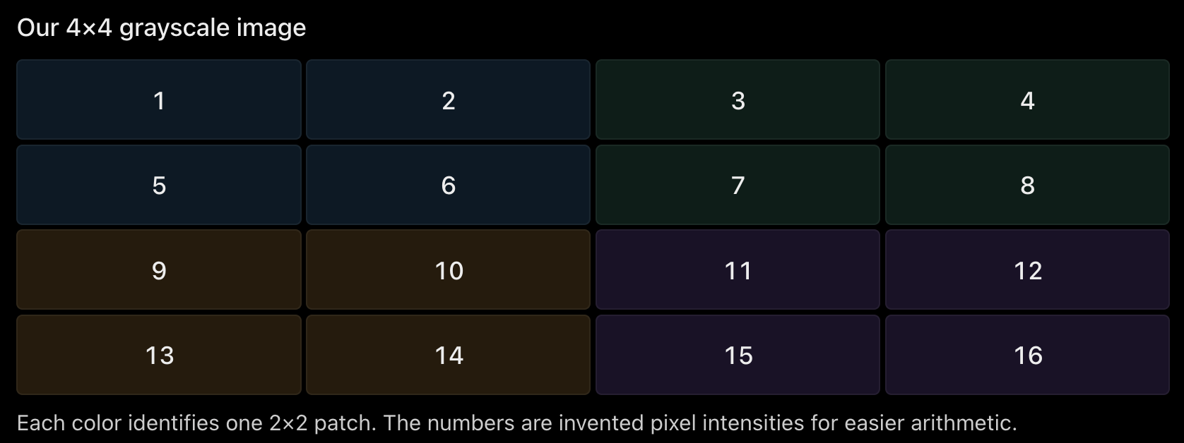
We get four patches.

Patch 1, top-left:

$$P_1 = \begin{bmatrix} 1 & 2 \ 5 & 6 \end{bmatrix}$$

Patch 2, top-right:

$$P_2 = \begin{bmatrix} 3 & 4 \ 7 & 8 \end{bmatrix}$$

Patch 3, bottom-left:

$$P_3 = \begin{bmatrix} 9 & 10 \ 13 & 14 \end{bmatrix}$$

Patch 4, bottom-right:

$$P_4 = \begin{bmatrix} 11 & 12 \ 15 & 16 \end{bmatrix}$$

Now, we're going to do something familiar from token embeddings: turn each patch into a vector.

Flatten each patch

Flattening means rearranging its values into a single sequence.

For Patch 1:

$$\begin{bmatrix} 1 & 2 \ 5 & 6 \end{bmatrix} \longrightarrow [1, 2, 5, 6]$$

Similarly:

$$P_2 = [3, 4, 7, 8]$$

$$P_3 = [9, 10, 13, 14]$$

$$P_4 = [11, 12, 15, 16]$$

Stacking all patches:

$$X_{\text{patches}} = \begin{bmatrix} 1 & 2 & 5 & 6 \ 3 & 4 & 7 & 8 \ 9 & 10 & 13 & 14 \ 11 & 12 & 15 & 16 \end{bmatrix}$$

Its shape is:

$$\boxed{[4, 4]}$$

Four patches, four pixel values per patch.

PyTorch: Extract patches

import torch
import torch.nn.functional as F

image = torch.arange(
    1, 17, dtype=torch.float32
).reshape(1, 1, 4, 4)

print(image.shape)
# torch.Size([1, 1, 4, 4])

patches = F.unfold(
    image,
    kernel_size=2,
    stride=2
)

print(patches.shape)
# torch.Size([1, 4, 4])

Why [1,4,4]?

F.unfold outputs:

$$[B,C\times P^2,N]$$

In our example:

• Batch size \(B=1\)
• Channels \(C=1\)
• Patch size \(P=2\)
• Number of patches \(N=4\)

So:

$$[1,1\times2\times2,4]=[1,4,4]$$

Let's transpose the last two dimensions so each row represents one patch:

patches = patches.transpose(1, 2)

print(patches[0])

Output:

tensor([[ 1.,  2.,  5.,  6.],
        [ 3.,  4.,  7.,  8.],
        [ 9., 10., 13., 14.],
        [11., 12., 15., 16.]])

This is exactly the matrix we calculated manually.

But here's the critical question:

Are these flattened pixel vectors already image embeddings?

Not in the semantic sense we want. They're raw pixel patches, rearranged into vectors. They haven't learned what features matter for understanding an image.

To produce useful patch embeddings, we need a learnable transformation.

How do pixel patches become learned embeddings?

Introduce a linear projection layer

Remember our discussion at the end of Module 1?

We learned that nn.Linear() can transform vectors from one representation space into another. We'll use exactly the same idea here.

Our patch matrix has shape:

$$X_{\text{patches}} : [4, 4]$$

We want each patch to become a two-dimensional embedding, purely for this example.

So we need a projection matrix:

$$W : [4, 2]$$

Then:

$$\boxed{E_{\text{patches}} = X_{\text{patches}} W}$$

The output shape is:

$$[4, 4] \times [4, 2] = \boxed{[4, 2]}$$

We now have four patch embeddings, each with two features.

Let's calculate one patch manually.

Take our first patch:

$$P_1 = [1, 2, 5, 6]$$

Suppose our projection matrix is:

$$W = \begin{bmatrix} 0.25 & 1 \ 0.25 & 0 \ 0.25 & 0 \ 0.25 & -1 \end{bmatrix}$$

Then:

$$e_1 = P_1 W$$

Calculate the first output feature:

$$e_{1,0} = 1(0.25) + 2(0.25) + 5(0.25) + 6(0.25)$$

$$\boxed{e_{1,0} = 3.5}$$

Calculate the second output feature:

$$e_{1,1} = 1(1) + 2(0) + 5(0) + 6(-1)$$

$$\boxed{e_{1,1} = -5}$$

Therefore:

$$\boxed{e_1 = [3.5, -5]}$$

Notice what happened.

We started with four pixel values:

$$[1, 2, 5, 6]$$

And converted them into two numerical features:

$$[3.5, -5]$$

In real vision models, the projection weights are learned from training, not manually defined.

PyTorch: Patch projection

import torch
import torch.nn as nn

projection = nn.Linear(
    in_features=4,
    out_features=2,
    bias=False
)

# Set our own weights for this teaching example
with torch.no_grad():
    projection.weight.copy_(torch.tensor([
        [0.25, 0.25, 0.25, 0.25],
        [1.00, 0.00, 0.00, -1.00]
    ]))

# patches is [1, 4, 4] from Batch 2
patch_embeddings = projection(patches)

print(patch_embeddings.shape)
# torch.Size([1, 4, 2])

print(patch_embeddings[0])

Output:

tensor([[ 3.5000, -5.0000],
        [ 5.5000, -5.0000],
        [11.5000, -5.0000],
        [13.5000, -5.0000]], grad_fn=<SelectBackward0>)

We now have a sequence of four patch embeddings.

Connection to text embeddings

Remember nn.Embedding?

For text:

token_embedding = nn.Embedding(
    num_embeddings=10000,
    embedding_dim=768
)

It looks up a learned vector using an integer token ID.

For images:

patch_embedding = nn.Linear(
    in_features=768,
    out_features=768
)

It computes a learned transformation of the actual pixel values within a patch.

These are different operations.

Text token embedding	Image patch embedding
Input is a discrete token ID	Input is a vector of pixel values
Retrieves a row from a learned table	Applies a learned linear projection
Same token ID initially produces the same vector	Different pixel patterns can produce different vectors
Shape [B,S] → [B,S,d]	Shape [B,N,CP²] → [B,N,d]

This is an important distinction for interviews.

What happens with a real RGB image?

Let's return to our 224×224 image.

We have:

$$C = 3, \quad H = W = 224$$

Patch size:

$$P = 16$$

How many pixel values exist inside one patch?

$$C \times P \times P$$

$$= 3 \times 16 \times 16$$

$$\boxed{768}$$

So each flattened RGB patch contains 768 numbers.

The image contains 196 patches.

After extraction:

$$\boxed{X_{\text{patches}}:[196,768]}$$

Suppose we choose a model hidden dimension of 768. Our learned projection is:

$$W:[768,768]$$

Therefore:

$$[196,768]\times[768,768]$$

$$\boxed{E_{\text{patches}}:[196,768]}$$

We've converted a 224×224 image into 196 learned patch tokens, each containing 768 features.

Now you may ask that the input patch dimension and output embedding dimension both happen to be 768. Does that mean projection is unnecessary?

The answer is No.

Just as we learned in Module 1, a projection can transform a representation even when its input and output dimensions match.

Also, the hidden dimension is a design choice. It doesn't have to equal the number of values inside a patch.

For instance, our 768-value patch could be projected into 512 or 1,024 dimensions.

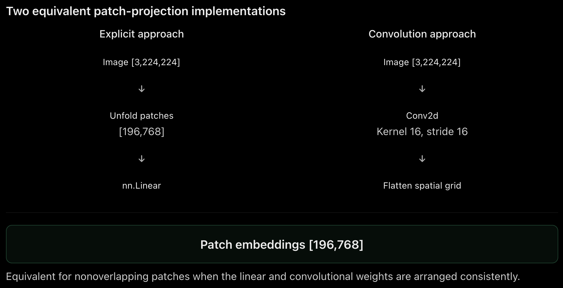
Why does ViT often use Conv2d for patch embeddings?

Here's something interesting.

We manually performed two steps:

1. Extract and flatten every image patch.
2. Apply the same linear projection to every patch.

These operations can be implemented together using a convolution.

For nonoverlapping square patches:

patch_embed = nn.Conv2d(
    in_channels=3,
    out_channels=768,
    kernel_size=16,
    stride=16
)

Why does that work?

A convolution kernel of size 16×16 covers one patch at a time.

With stride 16, it moves to the next nonoverlapping patch.

Each output channel has a learned set of weights covering all three input channels and the 16×16 spatial region.

So, at every patch location, it effectively computes a linear projection of 768 input pixel values into 768 output features.

PyTorch: Verify the convolution approach

Use our earlier tiny grayscale image and its projection weights.

conv = nn.Conv2d(
    in_channels=1,
    out_channels=2,
    kernel_size=2,
    stride=2,
    bias=False
)

# Copy the linear projection's weights into Conv2d
with torch.no_grad():
    conv.weight.copy_(
        projection.weight.reshape(2, 1, 2, 2)
    )

conv_output = conv(image)

print(conv_output.shape)
# [1, 2, 2, 2]

conv_tokens = conv_output.flatten(2).transpose(1, 2)

print(conv_tokens.shape)
# [1, 4, 2]

print(torch.allclose(conv_tokens, patch_embeddings))
# True

Here, flatten(2) combines the two spatial dimensions, and transpose(1,2) moves the channel dimension to the end.

We're left with [batch, number_of_patches, embedding_dimension].

So both approaches implement the same mathematical operation for this setup.

But Wait...haven't we lost the original image layout?

This is a very important question. After patch extraction, the model receives a sequence:

$$[P_1,P_2,P_3,\ldots,P_{196}]$$

But an image is not merely a collection of objects.Spatial relationships matter.

Consider these two situations:

• A person is standing above a staircase.
• A person is standing below a staircase.

If we shuffle the patches, the image changes drastically.

Yet standard self-attention, without any positional information, has no inherent understanding of which patch came from the top-left, center, or bottom-right.

The attention operation is permutation-equivariant over its input sequence in the absence of positional information.

In other words, rearranging patch tokens rearranges the corresponding outputs rather than giving the model an independent representation of the original layout.

Solution: Add positional embeddings

This should sound familiar from our text Transformer lessons. For every image patch, we provide positional information.

Suppose:

$$e_i = \text{PatchEmbedding}(P_i)$$

We add a positional vector:

$$p_i = \text{PositionEmbedding}(i)$$

Then:

$$\boxed{z_i = e_i + p_i}$$

Both vectors must have the same dimensionality. For example:

$$e_i = [0.2, 0.8]$$

$$p_i = [0.1, -0.3]$$

Then:

$$z_i = [0.3, 0.5]$$

This updated representation contains a combination of patch content and positional information.

PyTorch: Add learned positions

# Suppose 196 patches, each represented by 768 features

patch_tokens = torch.randn(1, 196, 768)

position_embeddings = nn.Parameter(
    torch.randn(1, 196, 768) * 0.02
)

tokens_with_position = (
    patch_tokens + position_embeddings
)

print(tokens_with_position.shape)
# [1, 196, 768]

The shape remains unchanged.

Some Vision Transformers use learned absolute positional embeddings; others use relative positional biases, rotary embeddings, or other positional mechanisms.

The central idea is the same: the model needs access to spatial relationships, not just patch content.

How do patch embeddings enter a Vision Transformer?

We're now very close to the familiar Transformer architecture. Remember the text-processing pipeline:

$$\text{Token Embeddings} \rightarrow \text{Positional Information} \rightarrow \text{Transformer Blocks}$$

A standard Vision Transformer follows a similar approach.

$$\text{Patch Embeddings} \rightarrow \text{Positional Information} \rightarrow \text{Transformer Blocks}$$

One common ViT design also introduces a learnable special token called the CLS token, or classification token.

Let's understand why.

What is the CLS token?

After patch extraction, we have:

$$X : [196, 768]$$

Each row represents one image patch. But suppose we want to represent the entire image using one vector.

One approach is to introduce an additional learned vector at the beginning of the patch sequence:

$$e_{\text{CLS}} \in \mathbb{R}^{768}$$

Our sequence becomes:

$$[\text{CLS}, P_1, P_2, \ldots, P_{196}]$$

Now the sequence contains 197 tokens. Therefore:

$$\boxed{X : [197, 768]}$$

During bidirectional self-attention, the CLS position can exchange information with the patch positions. After several Transformer blocks, its final hidden representation can be used as a summary of the image.

The CLS token isn't a manually calculated average. It's a learnable token whose representation evolves through attention and other Transformer operations.

Its usefulness as an image-level representation depends on the model's training.

How does self-attention work over image patches?

Once patches are projected into hidden vectors, the Transformer mathematics is very similar.

Suppose we have four patch embeddings:

$$X \in \mathbb{R}^{4 \times 8}$$

Using the learned projection matrices:

$$Q = X W_Q$$

$$K = X W_K$$

$$V = X W_V$$

The attention operation is:

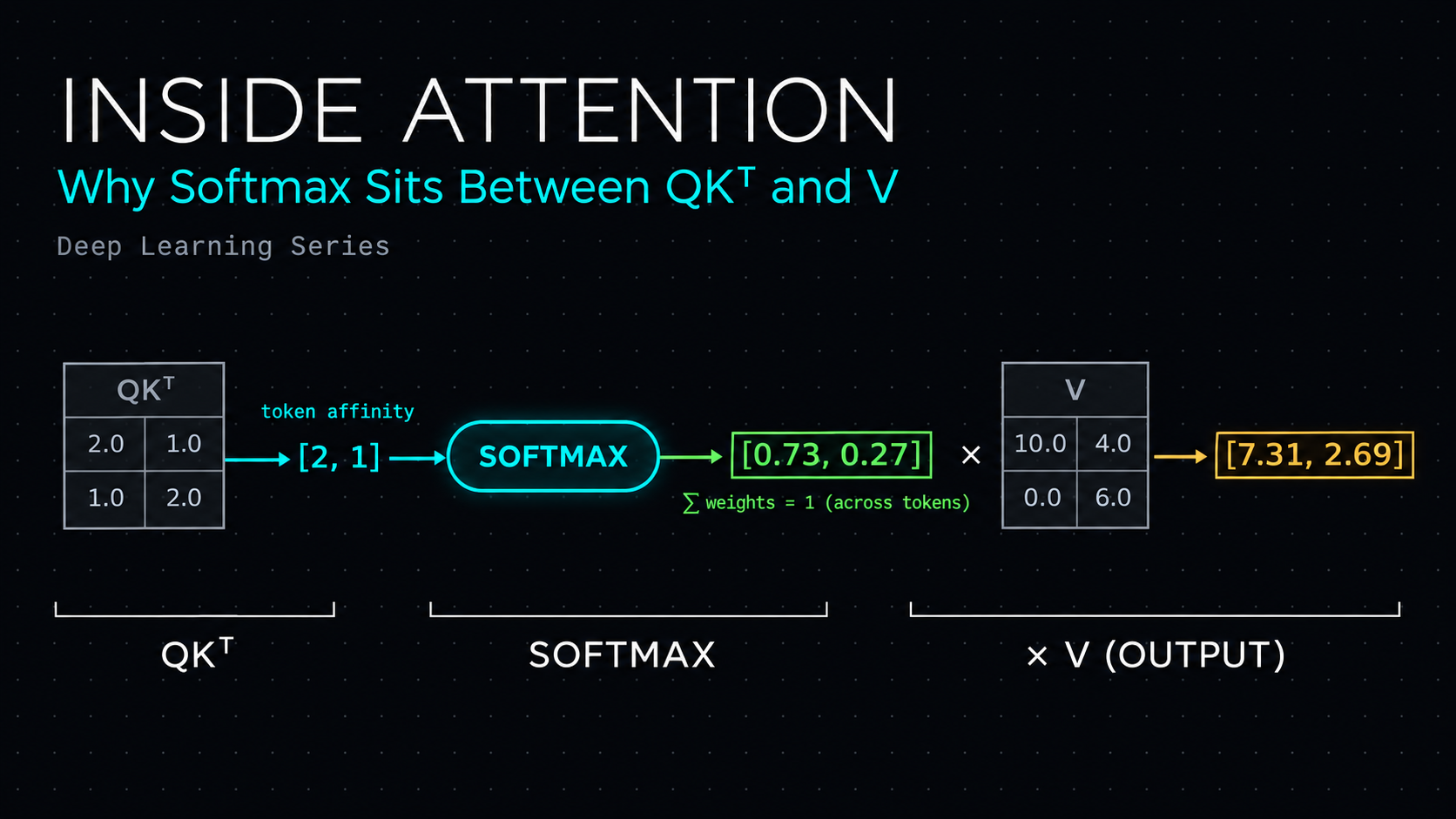
$$\boxed{ \operatorname{Attention}(Q, K, V) = \operatorname{softmax}\left( \frac{Q K^\top}{\sqrt{d_k}} \right) V }$$

The difference is that each row of $X$ represents an image patch rather than a text token.

Example

Imagine an image containing a dog on grass.

A patch showing part of the dog's face might benefit from information in patches showing the dog's body.

A patch containing grass might interact with other background patches.

Attention provides a mechanism for exchanging information between spatial regions.

But remember: attention isn't manually programmed to find dog faces or body parts.

Those patterns can emerge from training, depending on the architecture, data, and objective.

What is the attention matrix shape?

With 196 patch tokens and no CLS token:

$$QK^\top:[196,196]$$

Including CLS:

$$\boxed{QK^\top:[197,197]}$$

This is the matrix for one attention head, for one image.

Each row contains compatibility scores between one Query position and all 197 Key positions.

Unlike a causal text decoder, a typical ViT encoder permits bidirectional attention across image patches.

Why? When analyzing a complete image, the entire image is already available. There's usually no need to hide patches at later positions merely because they appear later in the flattened sequence.

Masked-image modeling is a different training setup and may deliberately hide visual content.

Build a tiny Vision Transformer from scratch

Now let's combine everything we've learned.

Our model will:

1. Accept an RGB image.
2. Convert it into patch embeddings using Conv2d.
3. Add a CLS token and positional embeddings.
4. Process the sequence through Transformer blocks.
5. Extract one image representation.
6. Project and normalize it to produce an image embedding.

We'll use a 16×16 image and 4×4 patches to keep the example small.

PyTorch: Build the model

import torch
import torch.nn as nn
import torch.nn.functional as F

class TinyVisionTransformer(nn.Module):

    def __init__(self):
        super().__init__()

        self.patch_size = 4
        self.hidden_dim = 32

        # 16x16 image with 4x4 patches = 16 patches
        self.num_patches = 16

        # Step 1: Patch embedding
        self.patch_embed = nn.Conv2d(
            in_channels=3,
            out_channels=32,
            kernel_size=4,
            stride=4
        )

        # Step 2: Learnable CLS token
        self.cls_token = nn.Parameter(
            torch.zeros(1, 1, 32)
        )

        # Step 3: Positional embeddings
        self.pos_embedding = nn.Parameter(
            torch.randn(1, 17, 32) * 0.02
        )

        # Step 4: Transformer encoder
        encoder_layer = nn.TransformerEncoderLayer(
            d_model=32,
            nhead=4,
            dim_feedforward=64,
            dropout=0.0,
            batch_first=True
        )

        self.transformer = nn.TransformerEncoder(
            encoder_layer,
            num_layers=2
        )

        # Step 5: Output projection
        self.projection = nn.Linear(32, 16)

    def forward(self, images):

        batch_size = images.shape[0]

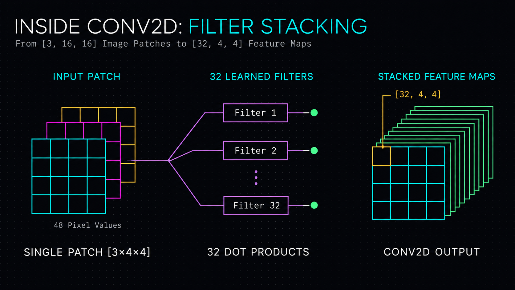
        # [B, 3, 16, 16] -> [B, 32, 4, 4]
        x = self.patch_embed(images)

        # [B, 32, 4, 4] -> [B, 16, 32]
        x = x.flatten(2).transpose(1, 2)

        # [1, 1, 32] -> [B, 1, 32]
        cls = self.cls_token.expand(
            batch_size, -1, -1
        )

        # [B, 16, 32] -> [B, 17, 32]
        x = torch.cat([cls, x], dim=1)

        # Add positional embeddings
        x = x + self.pos_embedding

        # Contextualize all tokens
        hidden_states = self.transformer(x)

        # Extract CLS representation
        image_representation = hidden_states[:, 0, :]

        # [B, 32] -> [B, 16]
        image_embedding = self.projection(
            image_representation
        )

        # L2 normalization
        image_embedding = F.normalize(
            image_embedding,
            dim=-1
        )

        return image_embedding

Run an image through the model

torch.manual_seed(42)

model = TinyVisionTransformer()
model.eval()

# Batch of two simulated RGB images
images = torch.randn(2, 3, 16, 16)

with torch.no_grad():
    embeddings = model(images)

print(embeddings.shape)
# torch.Size([2, 16])

print(embeddings.norm(dim=-1))
# tensor([1., 1.])

We've successfully created one 16-dimensional vector for each image.

Track the shapes through the complete model

Step	Tensor shape
Input images	[2, 3, 16, 16]
After convolution	[2, 32, 4, 4]
Patch token sequence	[2, 16, 32]
After adding CLS token	[2, 17, 32]
After positional embeddings	[2, 17, 32]
After Transformer blocks	[2, 17, 32]
CLS hidden representation	[2, 32]
Final image embeddings	[2, 16]

These shapes are worth understanding rather than memorizing.

How does the image encoder learn meaningful representations?

This is where Module 2 connects directly to Module 1.

Suppose we're training a CLIP-like text-image embedding system.

We prepare pairs such as:

Text	Image
"A dog running on grass"	Image of a running dog
"A red sports car"	Image of a red car
"A person holding an umbrella"	Image of a person with an umbrella

We pass the images through our image encoder and the captions through a text encoder. The two encoder outputs need compatible dimensions, possibly using projection layers.

We then calculate a similarity matrix:

$$S=E_{\text{text}}E_{\text{image}}^\top$$

Assuming embeddings are normalized, this gives pairwise cosine similarities.

Then we calculate a contrastive loss.

Gradients flow backward through the image projection, the Vision Transformer blocks, the patch projection, and, where learned, positional and CLS embeddings.

The image encoder learns representations that improve similarity-based ranking of matching images and text.

One final conceptual distinction

We've now encountered three different kinds of representations. It's important not to confuse them.

Representation	What it contains	Example shape
Flattened image patches	Raw pixel values within each patch	[196, 768]
Patch embeddings	Learned projections of individual patches	[196, 768]
Contextual patch representations	Patch vectors after self-attention and Transformer processing	[196, 768]
Final image embedding	One vector representing the complete image	[768]

These examples use the same 768-dimensional size for patch inputs, hidden states, and final outputs, but a real architecture may use different dimensions.

The crucial progression is:

$$\boxed{ \text{Pixels} \rightarrow \text{Patches} \rightarrow \text{Patch Embeddings} \rightarrow \text{Contextual Representations} \rightarrow \text{Image Embedding} }$$

And when paired with a text encoder and suitable training:

$$\boxed{ \text{Image Embedding} \leftrightarrow \text{Text Embedding} }$$

This is the foundation of text-to-image retrieval.

Module 2 recap

We've now opened up the image encoder rather than treating it as a black box.

We learned that:

• Images begin as tensors of pixel values.
• Vision Transformers commonly divide images into patches to reduce sequence length.
• Each patch is flattened and transformed into a learned embedding.
• Conv2d with matching kernel size and stride can efficiently implement nonoverlapping patch projection.
• Positional information helps preserve spatial relationships.
• Self-attention allows image patches to exchange information.
• A CLS token, mean pooling, or another aggregation mechanism can produce a single image representation.
• Training objectives determine whether that final vector becomes semantically useful.