Understanding LLM Embeddings from Scratch — Part 6: Static vs Contextual Embeddings (Self-Attention Explained)

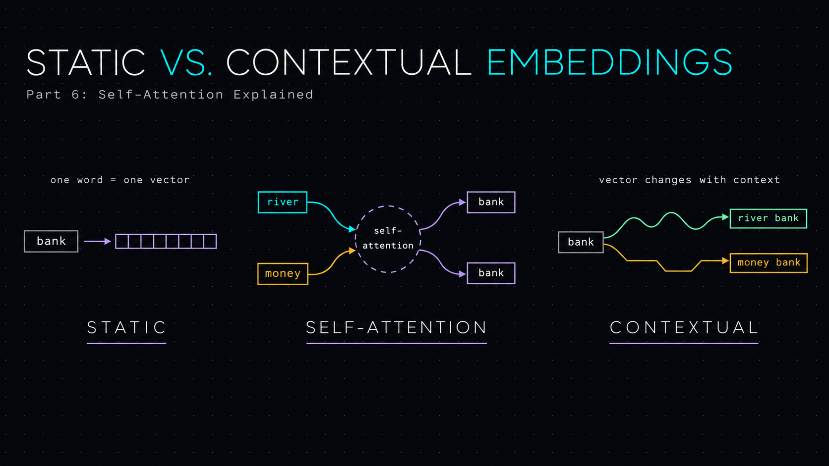
How does the same token represent different meanings in different sentences? Let's work through self-attention from first principles, with actual numbers and PyTorch.

In Part 5: Word2Vec, we saw how words that appear in similar contexts can develop similar vector representations. But Word2Vec-style embeddings have a limitation: once a word has been assigned a vector, that vector is the same regardless of the sentence.

Consider two short phrases:

river bank

money bank

We know that bank refers to two different things. But an embedding lookup only sees a token ID. If bank has the same token ID in both phrases, it retrieves the same row from the embedding matrix.

So where does the context come from?

That's the problem self-attention helps solve. In this part, we'll build it up from matrices, dot products, and softmax before seeing how the same starting embedding produces two different outputs.

1. The problem with a static token embedding

Let's start with a tiny vocabulary.

Token	Token ID	Embedding
river	0	[2.0, 0.0]
money	1	[0.0, 2.0]
bank	2	[1.0, 0.0]

For both phrases, the input embedding of bank is:

$$x_{\text{bank}}=[1,0]$$

The model isn't changing that stored row every time somebody types a new sentence. It needs to compute a new representation of the token occurrence, using the other tokens in the input.

One useful distinction:

• Input token embedding: a learned lookup vector for a token ID.
• Contextual hidden state: a representation computed using the token and whichever other token positions the model is allowed to access.

In a causal decoder-only LLM, a position can use its preceding tokens and itself, but not future positions.

2. First, start with some example matrix

We've already learned that individual tokens have embedding vectors. We can stack those vectors as rows of a matrix.

For river bank:

$$x_{\text{river}}=[2,0],\qquad x_{\text{bank}}=[1,0]$$

$$X=\begin{bmatrix}2&0\1&0\end{bmatrix}$$

Here its shape is [sequence_length, embedding_dimension] = [2, 2].

import torch
import math

torch.set_printoptions(precision=4)

X = torch.tensor([
    [2.0, 0.0],  # river
    [1.0, 0.0]   # bank
])

print(X.shape)  # torch.Size([2, 2])

For a model processing 2,048 token positions with a hidden dimension of 4,096, this X would have shape [2048, 4096]. If we batch several sequences together, we get a 3D tensor: [batch, sequence, hidden_dimension].

3. What are Query, Key, and Value?

Self-attention makes three different projections of the input:

$$Q=XW_Q,\qquad K=XW_K,\qquad V=XW_V$$

The three matrices \(W_Q\), \(W_K\), and \(W_V\) contain learned parameters. The same projections are applied to all positions in the sequence.

A useful intuition is:

Representation	Role
Query (Q)	What information is this position looking for?
Key (K)	What features can this position be matched on?
Value (V)	What information can this position contribute?

These descriptions are analogies. In the implementation, Q, K, and V are just vectors produced by matrix multiplication.

I would suggest to also read this blog: https://arpitbhayani.me/blogs/qkv-matrices/

Now, to simplify the first calculation, let's use the identity matrix:

$$I=\begin{bmatrix}1&0\0&1\end{bmatrix}$$

Multiplying a compatible matrix by the identity leaves it unchanged: \(XI=X\).

If we deliberately set \(W_Q=W_K=W_V=I\), then:

$$\boxed{Q=K=V=X}$$

I = torch.eye(2)
W_Q = W_K = W_V = I

Q = X @ W_Q
K = X @ W_K
V = X @ W_V

print(Q)
print(K)
print(V)
# All three are [[2., 0.], [1., 0.]]

Important: We are using identity matrix only for teaching shortcut. A trained Transformer almost always has different Q, K, and V projections. The output dimensions can also differ from the input embedding dimension.

q_bank  = Q[1]  # [1., 0.]
k_river = K[0]  # [2., 0.]
k_bank  = K[1]  # [1., 0.]

v_river = V[0]  # [2., 0.]
v_bank  = V[1]  # [1., 0.]

4. How does the bank position compare itself with other tokens?

Attention compares a position's Query with other positions' Keys using the dot product.

For bank querying river:

$$q_{\text{bank}}\cdot k_{\text{river}}=[1,0]\cdot[2,0]=1(2)+0(0)=2$$

For bank querying itself:

$$q_{\text{bank}}\cdot k_{\text{bank}}=[1,0]\cdot[1,0]=1$$

In Python:

print(torch.dot(q_bank, k_river))  # tensor(2.)
print(torch.dot(q_bank, k_bank))   # tensor(1.)

What if we want all query-key comparisons at once? Stack them and use matrix multiplication.

$$QK^T=\begin{bmatrix}2&0\1&0\end{bmatrix}\begin{bmatrix}2&1\0&0\end{bmatrix}=\begin{bmatrix}4&2\2&1\end{bmatrix}$$

The transpose (\(K^T\)) swaps the rows and columns so that each query is compared with every key.

raw_scores = Q @ K.T
print(raw_scores)
# tensor([[4., 2.],
#         [2., 1.]])

How to read this matrix: rows are query positions; columns are key positions. The second row [2, 1] contains the scores for the bank query against river and bank.

5. Why divide by the square root of the Key dimension?

Transformers use scaled dot-product attention:

$$S=\frac{QK^T}{\sqrt{d_k}}$$

Our Keys have two coordinates, so \(d_k=2\) and \(\sqrt{2}\approx1.4142\).

$$S\approx\begin{bmatrix}2.8284&1.4142\1.4142&0.7071\end{bmatrix}$$

d_k = K.shape[-1]  # 2
scores = raw_scores / math.sqrt(d_k)
print(scores)

Why do we scale? Under common assumptions about the components of Q and K, the variance of an unscaled dot product grows with the dimension. Large scores can make softmax extremely peaked, potentially producing small gradients. Scaling helps control that effect.

6. Why do we need a causal mask?

A decoder-only LLM must not peek at future tokens when predicting the next token.

For river bank:

Query ↓ / Key →	river	bank
river	Allowed	Blocked
bank	Allowed	Allowed

We implement this by adding negative infinity to disallowed attention scores before softmax:

$$M=\begin{bmatrix}0&-\infty\0&0\end{bmatrix}$$

future_mask = torch.triu(
    torch.ones(2, 2, dtype=torch.bool),
    diagonal=1
)

masked_scores = scores.masked_fill(
    future_mask, float('-inf')
)

print(masked_scores)
# tensor([[2.8284,   -inf],
#         [1.4142, 0.7071]])

Since \(\exp(-\infty)=0\), a masked position gets zero attention weight after softmax.

Don't confuse causal masks with padding masks. Causal masks block future positions; padding masks block artificial padding tokens. A Transformer may need both. Also, different PyTorch APIs use different conventions for boolean masks, so always check the documentation.

7. Softmax turns scores into attention weights

We have two valid scores for the bank query:

$$[1.4142,\ 0.7071]$$

Softmax converts these into nonnegative weights that sum to one:

$$\alpha_j=\frac{e^{s_j}}{\sum_k e^{s_k}}$$

For bank attending to river:

$$\alpha_{\text{river}}=\frac{e^{1.4142}}{e^{1.4142}+e^{0.7071}}\approx0.6698$$

And the remaining weight is:

$$\alpha_{\text{bank}}\approx0.3302$$

attention_weights = torch.softmax(
    masked_scores, dim=-1
)

print(attention_weights)
# tensor([[1.0000, 0.0000],
#         [0.6698, 0.3302]])

The first row attends 100% to river, because bank is in the future. The second row attends approximately 67% to river and 33% to itself.

8. Values: The actual information being combined

Attention isn't complete after calculating weights. Now the model combines the Value vectors.

$$o_i=\sum_j\alpha_{ij}v_j$$

For bank:

$$o_{\text{bank}}=0.6698v_{\text{river}}+0.3302v_{\text{bank}}$$

Remember: \(v_{\text{river}}=[2,0]\) and \(v_{\text{bank}}=[1,0]\).

$$o_{\text{bank}}=0.6698[2,0]+0.3302[1,0]$$

$$=[1.3396,0]+[0.3302,0]$$

$$\boxed{o_{\text{bank}}\approx[1.6698,0]}$$

In code, the calculation is just matrix multiplication:

output = attention_weights @ V

print(output)
# tensor([[2.0000, 0.0000],
#         [1.6698, 0.0000]])

This is the essential idea: the token position's output now incorporates information from other accessible token positions.

9. Same bank embedding, different contextual output

Now replace river with money:

$$X_{\text{money}}=\begin{bmatrix}0&2\1&0\end{bmatrix}$$

The initial embedding of bank is still [1, 0]. We haven't modified the embedding table.

Let's repeat the same attention calculation with identity projections:

X_money = torch.tensor([
    [0.0, 2.0],  # money
    [1.0, 0.0]   # bank
])

Qm = Km = Vm = X_money

scores_m = Qm @ Km.T / math.sqrt(2)
scores_m = scores_m.masked_fill(future_mask, float('-inf'))
weights_m = torch.softmax(scores_m, dim=-1)
output_m = weights_m @ Vm

print(weights_m)
# tensor([[1.0000, 0.0000],
#         [0.3302, 0.6698]])

print(output_m[1])
# tensor([0.6698, 0.6605])

Compare the outcomes:

Input	Initial embedding of bank	Attention output at bank
river bank	[1.0, 0.0]	[1.6698, 0.0000]
money bank	[1.0, 0.0]	[0.6698, 0.6605]

That's contextualization. The input embedding is shared, but the output depends on the sequence. Note that this is an attention sublayer output, not yet the final hidden state of an entire Transformer block.

10. The entire attention equation in one line

We can now combine every step into the full equation:

$$\boxed{\operatorname{Attention}(Q,K,V)=\operatorname{softmax}\left(\frac{QK^T}{\sqrt{d_k}}+M\right)V}$$

Read it from left to right:

1. \(QK^T\): compare every query with every key.
2. Divide by \(\sqrt{d_k}\): scale the scores.
3. Add M: block disallowed positions.
4. Softmax: get weights that sum to one.
5. Multiply by V: produce weighted combinations of values.

Our complete example becomes just a few lines:

Q, K, V = X @ W_Q, X @ W_K, X @ W_V
scores = Q @ K.T / math.sqrt(K.shape[-1])
scores = scores.masked_fill(future_mask, float('-inf'))
weights = torch.softmax(scores, dim=-1)
output = weights @ V

11. But real Q, K, and V aren't equal to X

We set \(W_Q=W_K=W_V=I\) so that we could see every numerical step. In a trained model, those projections have learned weights and different roles.

For example, if we change only the Value projection to:

$$W_V=\begin{bmatrix}0.5&0.2\0.3&0.8\end{bmatrix}$$

then:

W_V_new = torch.tensor([
    [0.5, 0.2],
    [0.3, 0.8]
])

V_new = X @ W_V_new
print(V_new)
# tensor([[1.0000, 0.4000],
#         [0.5000, 0.2000]])

new_output = attention_weights @ V_new
print(new_output[1])
# tensor([0.8349, 0.3340])

We changed the Values, so the resulting weighted information changes. The attention weights remain unchanged because Q and K haven't changed.

A full Transformer learns all three projections through gradient-based training, just as it learns its embedding matrix (Part 4).

12. What happens to the tensor shapes?

In practice, we don't calculate one Query at a time. We process whole sequences, often in batches.

Suppose:

• Batch size \(B=2\)
• Sequence length \(S=3\)
• Model dimension \(d_{model}=8\)
• One attention head, with \(d_k=d_v=8\)

Then:

Tensor	Shape
Input hidden states X	[2, 3, 8]
Q, K, V	[2, 3, 8]
\(QK^T\)	[2, 3, 3]
Attention weights	[2, 3, 3]
Attention output	[2, 3, 8]

13. Multi-head attention: More than one way to look at context

A real Transformer typically has multiple attention heads, not just one. Each head uses its own learned projections, creating its own attention pattern. The outputs are concatenated and passed through another projection \(W_O\).

For example, if \(d_{model}=8\) and there are two heads, a simple configuration uses four dimensions per head.

# Batch=2, sequence=3, model dimension=8
x = torch.randn(2, 3, 8)
q_linear = torch.nn.Linear(8, 8, bias=False)

q = q_linear(x)
q = q.reshape(2, 3, 2, 4).transpose(1, 2)

print(q.shape)
# torch.Size([2, 2, 3, 4])
# [batch, heads, sequence, head_dimension]

The conceptual advantage is that different heads can learn different patterns for finding and combining information.

14. Position matters too

What about these sentences?

dog bites man

man bites dog

An embedding lookup contains token identity, but doesn't by itself say where each token occurs. Attention needs positional information to distinguish ordering and relative positions.

One approach adds a positional vector to every token embedding:

$$x_i=e_i+p_i$$

Another widely used approach is Rotary Positional Embeddings (RoPE). You folks can also read about it.

Our two-token example omitted positional encoding intentionally.

15. A small trainable PyTorch experiment

Now let's connect the mathematics to the learning process from Part 4.

We'll train a tiny causal-attention model on two examples:

Input	Desired next token
river bank	shore
money bank	loan

The same bank embedding row is used in both examples. The output must depend on the preceding token.

Our toy model contains an input embedding layer, Q/K/V projections, causal attention, an output projection, a residual connection and layer normalization, and a vocabulary prediction head.

Here's the heart of the implementation:

import torch.nn as nn
import torch.nn.functional as F

class TinyCausalAttention(nn.Module):
    def __init__(self, vocab_size=5, dim=12):
        super().__init__()
        self.emb = nn.Embedding(vocab_size, dim)
        self.q = nn.Linear(dim, dim, bias=False)
        self.k = nn.Linear(dim, dim, bias=False)
        self.v = nn.Linear(dim, dim, bias=False)
        self.o = nn.Linear(dim, dim, bias=False)
        self.norm = nn.LayerNorm(dim)
        self.lm_head = nn.Linear(dim, vocab_size)
        self.dim = dim

    def forward(self, ids):
        X = self.emb(ids)
        Q, K, V = self.q(X), self.k(X), self.v(X)
        scores = Q @ K.transpose(-2, -1) / math.sqrt(self.dim)
        n = ids.shape[1]
        mask = torch.triu(torch.ones(n, n, dtype=torch.bool), diagonal=1)
        weights = torch.softmax(scores.masked_fill(mask, float('-inf')), dim=-1)
        hidden = self.norm(X + self.o(weights @ V))
        return self.lm_head(hidden)

Train it on our two pairs, using only the final position's logits:

torch.manual_seed(42)
model = TinyCausalAttention()

# 0 river, 1 money, 2 bank, 3 shore, 4 loan
inputs = torch.tensor([[0, 2], [1, 2]])
targets = torch.tensor([3, 4])

optimizer = torch.optim.Adam(model.parameters(), lr=0.03)
loss_history = []

for step in range(201):
    logits = model(inputs)[:, -1, :]
    loss = F.cross_entropy(logits, targets)
    loss_history.append(loss.item())

    optimizer.zero_grad()
    loss.backward()
    optimizer.step()

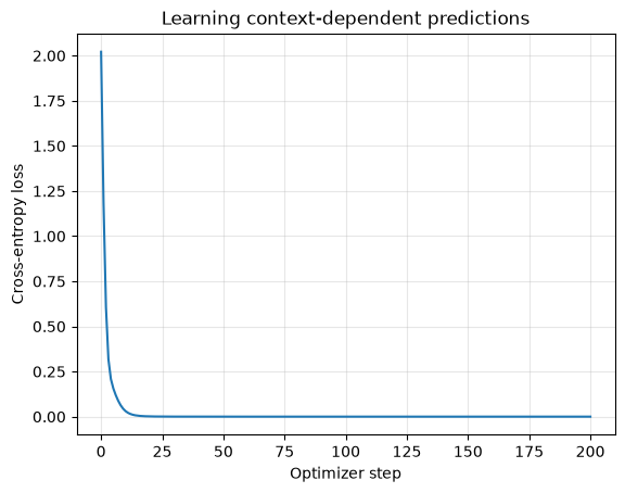
Plot the learning curve:

import matplotlib.pyplot as plt

plt.plot(loss_history)
plt.xlabel('Optimizer step')
plt.ylabel('Cross-entropy loss')
plt.title('Learning context-dependent predictions')
plt.grid(alpha=0.3)
plt.show()

16. Why this matters for inference engineering

Understanding Q, K, and V also explains an important inference optimization: KV caching.

During autoregressive generation, a new token needs to attend to earlier positions. The model can reuse previously computed Keys and Values for those positions instead of recomputing them in every decoding step.

It computes a new Query for the new position and compares it with cached Keys. Then it takes the weighted combination of cached Values (plus the new position's Value).

Why not cache previous Queries too? In ordinary causal decoding, old Queries aren't needed to compute the output for the newly generated position. The new Query is what needs to search past Keys.

This is also why sequence length affects KV-cache memory, and why multi-query and grouped-query attention can improve serving efficiency.

One more distinction: attention weights are not themselves a complete explanation of model behavior. Values, learned projections, residual paths, later Transformer blocks and the prediction head all contribute to the final answer.